doi:10.1016/j.jenvman.2005.08.007

Application of a system dynamics approach for assessment and mitigation

of CO

emissions from the cement industry

Shalini Anand

, Prem Vrat

, R.P. Dahiya

Centre for Energy Studies, Indian Institute of Technology Delhi, Hauz Khas, New Delhi 110016, India

Indian Institute of Technology Roorkee, Uttranchal-247667, India

Received 21 August 2003; revised 2 August 2005; accepted 3 August 2005

Available online 22 November 2005

Abstract

A system dynamics model based on the dynamic interactions among a number of system components is developed to estimate CO

emissions

from the cement industry in India. The CO

emissions are projected to reach 396.89 million tonnes by the year 2020 if the existing cement making

technological options are followed. Policy options of population growth stabilisation, energy conservation and structural management in cement

manufacturing processes are incorporated for developing the CO

mitigation scenarios. A 42% reduction in the CO

emissions can be achieved in

the year 2020 based on an integrated mitigation scenario. Indirect CO

emissions from the transport of raw materials to the cement plants and

ﬁnished product to market are also estimated.

Keywords: Cement industry; CO2 emissions; Greenhouse gases; Mitigation options; System dynamics

1. Introduction

Energy use in the industrial sector is responsible for

approximately one third of the global carbon dioxide (CO

)

emissions. In India, six industries have been identiﬁed as

energy-intensive, viz: aluminium, cement, fertilizer, iron and

steel, glass, and paper (Schumacher and Sathaye, 1999). The

cement sector holds a considerable share within these energy-

intensive industries. The CO

emissions from cement plants are

next only to the coal based thermal power plants. On the global

scale the cement industry is responsible for 20% of the man-

made CO

emissions. This contributes to around 10% of the

man-made global warming potential.

In cement making, nearly half of the carbon dioxide

emissions result from energy use and the other half from the

decomposition of calcium carbonate during clinker production

(Hendriks et al., 1999). Moreover, the transport of raw

materials and ﬁnished products indirectly contributes to the

share of CO

emission from the cement industry.

At present, the Indian cement industry produces 13 different

types of cement; out of which Ordinary Portland Cement

(OPC), Portland Pozzolana Cement (PPC) and Portland Slag

Cement (PSC) together constitute 99%. Two cement varieties

are in use, white and grey. OPC consists of 95% clinker and 5%

gypsum. PPC consists of 65% clinker, 5% gypsum and 30%

pozzolana. Pozzolana materials include volcanic ash, power-

station ﬂy ash, burnt clays, ash from burnt plant material and

silicious earths. Pozzolana has siliceous (SiO

) and aluminous

(Al

) materials that do not possess cementing properties but

develop these properties in the presence of water. It has a lower

heat of hydration, which h elps in preventing cracks where large

volumes are being cast. PSC consists of 30% clinker, 5%

gypsum and 65% slag. It has a heat of hydration even lower

than that of PPC and is generally used in the construction of

dams and similar massive structures (Worrell et al., 1995;

Karwa et al., 1998).

Limestone is a major raw material used in the production of

cement. It is burnt to make clinker and is blended with

additives. The ﬁnished product is then ﬁnely grounded to

produce different types of cement (World Energy Counci l,

1995; Schumacher and Sathaye, 1999). Additives used are

mainly ﬂy ash from coal-ﬁred thermal power plants, slag from

blast furnaces in the iron and steel industry, pozzolana and

natural zeolites. Natural zeolite contains large quantities of

reactive SiO

and Al

. Zeolite substitution can improve the

strength of concr ete by the pozzolanic reaction with Ca(OH)

This is a reaction in the presence of lime (calcium oxide, CaO)

and water to produce reaction products that are cementitious in

nature.

Journal of Environmental Management 79 (2006) 383–398

www.elsevier.com/locate/jenvman

doi:10.1016/j.jenvman.2005.08.007

Corresponding author.

In the cement production process around 0.97 tonne of CO

is produced for each tonne of clinker produc ed. Its distribution

is mainly from calcination (0.54 tonne), use of coal and fossil

fuels (0.34 tonne) and electricity generation (0.09 tonne)

(Marchal, 2001). On an average, around 900 kg of clinker is

used in each 1000 kg of cement produced. Thus each tonne of

cement is associated with 0.873 tonne of CO

emissions

(CE MBUREAU, 1996, 1998, 1999; International Energy

Agency, 1999; McCaffrey, 2001).

While working out the need for cement production in the

coming years, various policy options should be explored

keeping in view their environmental aspects. Implications of

the policy options and the associated dynamics of CO

emissions from the cement industry can be analysed using a

System Dynamics (SD) approach. In this dynamic simulation

approach information governing the interactions in a system is

fed via interactive feedback loops.

In management and social systems, policy-makers and

researchers have extensively used SD methodology and

conducted policy experiments (Mohapatra et al., 1994). The

SD approach has also been applied to a number of studies

related to the environment; environmental impact assessment

analysis (Vizayakumar and Mohapatra, 1991, 1993), solid

waste management (Mashayekhi, 1993; Karavezyris et al.,

2002), analysis of greenhouse gas emissions and global

warming (Naill et al., 1992; Vrat et al., 1993), investigations

of methane emissions from rice cultivation in the Indian

context (Anand et al., 2005), water resource planning (Ford,

1996), environmental planning and management (Guo et al.,

2001; Guneralp and Barlas, 2003), environmental sustain-

ability (Saysel et al., 2002), ecological modeling (Wu et al.,

1993) and many mor e situations. Though the SD model deals

with a system in an integrated sense, the system is decomposed

by dividing it into a number of interacting subsystems. The

individual subsystems can then be analysed and integrated

keeping the mutual interactions among the subsystems.

In this paper we have adopted the System Dynamics

methodology for assessment and mitigation of CO

emissions

from the cement industry in India. The projections of cement

production are considered to be mainly inﬂuenced by the

population growth, the gross domestic product (GDP)

increment rate and technologies employed in the cement

industry. A software package ‘Powersim’, which is available

for system dynamics analysis has been used in developing a

model for the cement sector. The proposed model is a

combination of spreadsheet (excel) and system dynamics

modeling framework. By interfacing the two the capabilities of

both are mutually reinforced, as there is dynamic exchange of

data during the course of simulation. Use of a spreadsheet gives

the ﬂexibility of manipulating some of the data before it is fed

into the system dynamics model, thus enhancing the scope of

policy experimentation.

2. System dynamics model for cement sector

In a system dynamics model, the simulations are essentially

time-step simulations. The model takes a number of simulation

steps along the time axis (Anand et al., 2005). The dynamics of

the system are represented by d N(t)/dtZkN(t), which has a

solution N(t)ZN

expt(kt). Here, N

is the initial value of the

system variable, k is a rate constant (which affects the state of

the system) and t is the simulation time. For the simulations to

start for the ﬁrst time, initial values of the system variables are

needed.

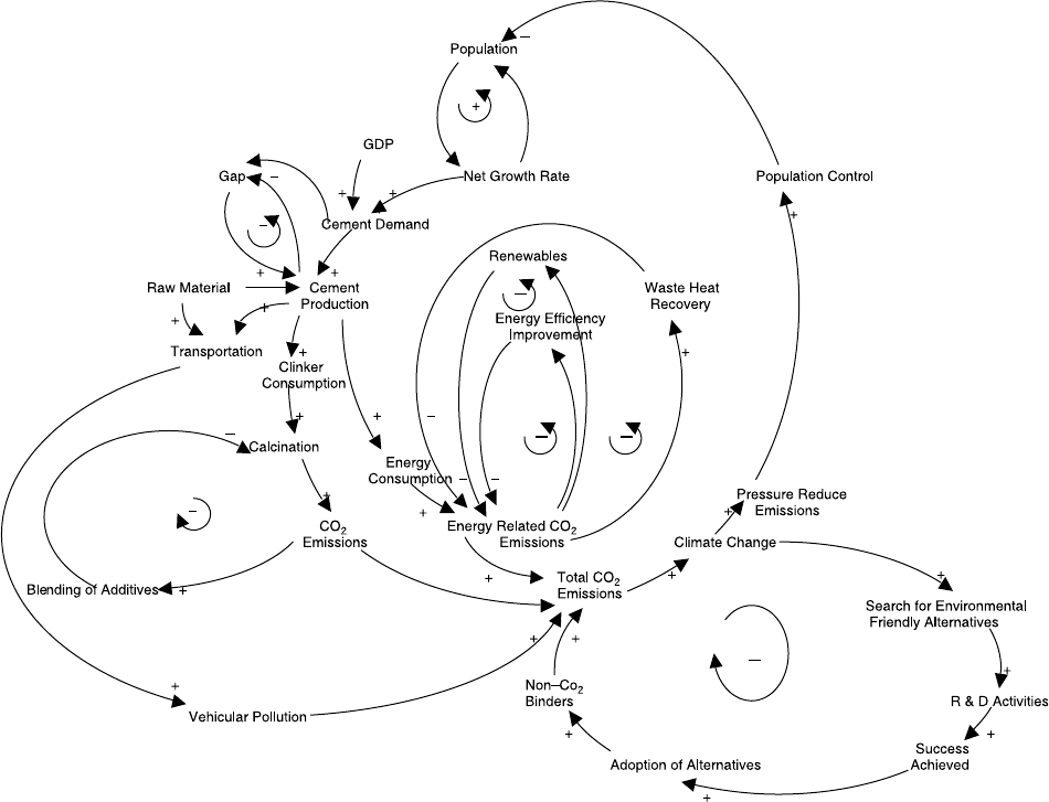
2.1. Causal loop diagram

The SD model for the present studies was developed for

scenario building, conducting policy experiments and making

projections for CO

emissions. A causal loop diagram, shown

in Fig. 1, was developed by incorporating the various features

associated with the cement sector. A ﬂow diagram was then

created from the causal loop diagram and dynamo equations for

each element in the diagram were added in the model. The

model so evolved was run for a period of 20 years starting from

the baseline year 2000.

The mutual interactions associated with cement production

and the related CO

emissions are qualitatively expressed in the

causal loop diagram. Dynamics of the model are determined by

the feedback loops of the causal loop diagram. Each arrow of

the causal loop diagram indicates the inﬂuence of one element

on the other. The inﬂuence is considered positive ( C )ifan

increase in one element causes an increase in another, or

negative (K) in the opposite case. The causal loop diagram is

self-explanatory.

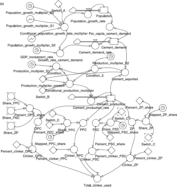
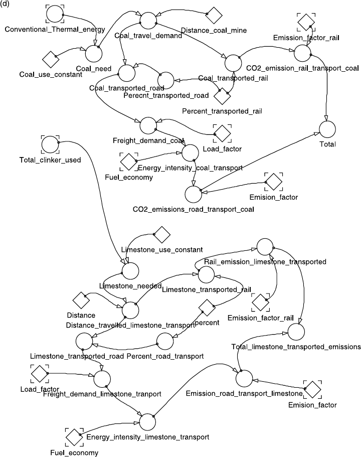
2.2. Flow diagram

A ﬂow diagram is useful for showing the physical and

information ﬂows in the SD model. Fig. 2a–e show the details

of the ﬂow diagram developed for anal ysing the cement sector.

Intricacies of the mutually interacting processes are delineated

in the ﬂow diagram.

The level variables are shown as rectangular boxes which

represent accumulated ﬂows to that level. A double arrow

represents the physical ﬂows, and the ﬂow is controlled by

a ﬂow rate. A single line is for showing information ﬂow.

Source and sink of the structure are represented by a cloud.

The cloud symbol indicates inﬁnity and marks the boundary

of the model.

Once the simulation is over, at the end of each step,

system variables are brought up to date for representing the

results from the previous simulation step. The rate variables

are represented by valves. The information from the level

variables to the rate variables is transformed by a third

variable called the auxiliary variable, represented by circles.

The diamonds represent constants, which do not vary over

the run period of simulation. A constant is deﬁned by an

initial value throughout the simul ation. To avoid messing up

and criss-crossing in the diagram the variables repeated in

the diagram are represent ed in the form of snapshot

variables (frame-like structures).

Five subsystems corresponding to different scenarios are

built and discussed in the following sections:

S. Anand et al. / Journal of Environmental Management 79 (2006) 383–398384

2.2.1. demand and production

Cement demand and production are taken as level variables.

The cement demand represented in Fig. 2(a) would increase with

the growth of population and the gross domestic product (GDP).

Production should follow the demand and the CO

emissions

from the plants would likewise increase with more production.

This requires information about population, and the population is

then considered as a level variable. Its variation obviously

depends on the rate of population growth. Percent share of

different varieties of cement are worked out and accordingly the

clinker consumed in cement production is estimated. Since

changes in population growth rate, cement production rate, and

percent share of blended cement affect the rate of CO

emissions

from the cement industry, the impact of these changes is tested

using an additional auxiliary named ‘switch’. The user can adjust

its value to select one of the possible options.

The dynamo equations used to account for the baseline

scenario (BS), scenarios 1 and 2 (S1 and S2) in this

subsystem are

Population Z Population C dt

!Population_growth_rate (1)

where

Population_growth_rate Z Population!Condi-

tional_population_-

growth_rate_multiplier

Conditional_population

_growth_rate_multiplier Z IF(Switch_AZ 1,

Population_growth_-

multiplier_BS, IF(Swi-

tcha _AZ 2,Popul-

tion_growth_multiplier

_S1,Population_gro-

wth_multiplier_S2))

Population_growth_multiplier_BS Z0.016CSTEP

(K.0003,2001)CSTEP

(K.0007,C2006 )C

STEP(K.0006,C2011)

Population_growth_multiplier_S1 Z GRAPH(TIME,

2000,1,[0.0162,0.0157,

0.0157,0.0148,0.0139,

0.013,0.0121,0. 0112,

0.0103,0.0094,0.0085,

0.0076,0.0067,0.0058,

0.0049,0.004,0. 0031,

0.0022,0.0013,0 ,

0”Min:0;Max:0.02”])

Fig. 1. Causal—loop diagram of the system dynamics model for cement sector.

S. Anand et al. / Journal of Environmental Management 79 (2006) 383–398 385

Population_growth_multiplier_S2 Z GRAPH(TIME,

2000,1,[0.0162,0.0157,

0.0157,0.0138,0.0119,

0.01,0.0081,0.0 062,

0.0043,0.0024,0.0005,

0,0,0,0,0,0,0,0 ,0,

0”Min:0;Max:0.02”])

For cement demand and production the dynamo

equations used in the model are as follows:

Cement_demand

Z Cement_demand C dt!Cement_demand_rate (2)

where

Cement_demand_rate ZGrowth_rate_cement

_demand!Cement_de-

mand

Growth_rate_cement_demand ZGDP_increament_ra-

teCConditional_popu-

lation_growth

rate_multiplier

and, therefore, cement demand can be expressed as

Cement_demand

Z Cement_demand C dt!fðGDP_increament_rate

C Conditional_population_growth_rate_multiplierÞ

!ðCement_demand_rateÞg (3)

Now,

Fig. 2. Flow diagrams of the system dynamics model for cement sector. Subsystem diagrams are labeled as Figs. a–e. Fig. 2 (a) Subsystem depicting the interactions

among population, cement demand, cement production and total clinker used. (b) Subsystem for evaluating the electric and thermal energy consumption and total

emissions. (c) Subsystem for incorporating the coal consumption, ﬂy ash production, pig iron production and slag availability. (d) Subsystem for estimating CO

emissions from transport of raw materials (limestone and coal) from their mines to the cement plants. (e) Subsystem for estimating CO

emissions due to the

transport of cement to market.

S. Anand et al. / Journal of Environmental Management 79 (2006) 383–398386

Cement_production

Z Cement_production C dt

!Cement_production_rate (4)

Cement_exported

Z Cemnent_productionKCement_demand (5)

where,

Cement_production_rate Z Cemen t_produc-

tion!Conditional_pro-

duction_multiplier

Conditional_production

_multiplier Z IF(Switch_BZ 1,

Production_multiplier_

present, IF(Switch_BZ

2, Condition_1,

Condition_2))

Condition_1 ZIF(Cement_exported

O0, Production_multi-

plier_S1, Production_-

multiplier_present)

Condition_2 ZIF(Cement_exported

O0, Production_multi-

plier_S2, Production

_multiplier_present

Fig. 2 (continued)

S. Anand et al. / Journal of Environmental Management 79 (2006) 383–398 387

where the production_multiplier_present is for the base-

line scenario.

Similarly, the dynamo equations were written for energy

consumption, availability of slag and ﬂy ash, CO

emissions

from cement plants and CO

emissions arising from transport

requirements.

2.2.2. Energy consumption

Electric energy consumption for the cement industry is

estimated by considering the electric energy consumed per

tonne of cement produced. Its ﬂow diagram is shown in Fig. 2

(b). For the various policy options it is bifurcated into the

conventional electric energy and electric energy from renew-

ables. The share of these is varied by a switch function for

alternate scenarios. Similarly, the thermal energy consumption

is estimated by taking into account the thermal energy

consumed per tonne of clinker used. Scenarios considering

improved thermal energy efﬁciency and waste heat recovery

are also evaluated under this head.

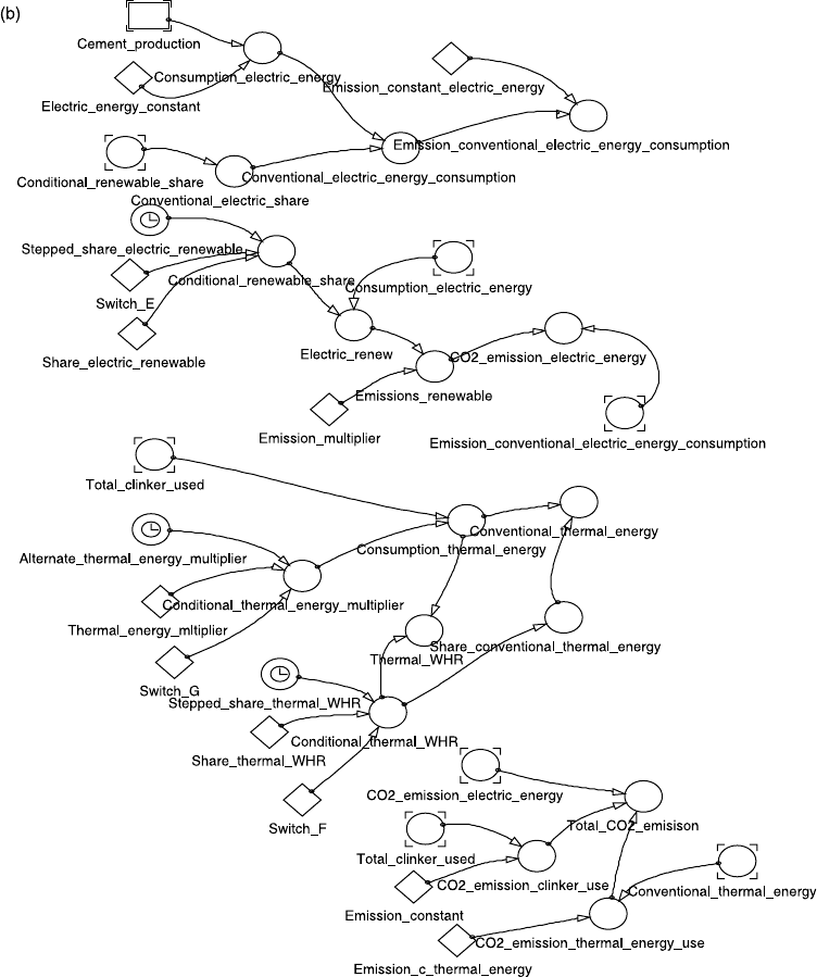
2.2.3. Avalability of slag and ﬂy ash

The ﬂow diagram shown in Fig. 2 (c) is used to estimate the

availability of the blending materials, i.e. slag, ﬂy ash and

zeolite. Coal consumption for power generation, taken as a

level variable, is calculated and projected for a span of 20

years. For estimating the availability of ﬂy ash it is assumed

that on an average the Indian coal has 33% ash content (Mehra

and Damoda ran, 1993; Choudhary and Bhakatvatsalam, 1997;

www.cea-in/opt7-vidyut-chap4.html). Out of this 80% comes

out as ﬂy ash during coal combustion in thermal power plants.

Approximately, 50% of the wet ﬂy ash disposed in the ash

ponds is suited for cement making (Worrell et al., 1995) and

the dried ﬂy ash can be lifted from the ash ponds.

Slag is produced in the blast furnace of pig iron plants. In

this process 0.7 tonne of slag is gener ated per tonne of pig iron

produced (Worrell et al., 1995).

2.2.4. CO

emissions from cement plants

Total CO

emissions from cement plants are estimated as

the sum total of CO

emissions from the consumption of

clinker in the process of thermal energy production and

generation of electric energy required for the plants. Policy

options are implemented while working out the scenarios for

the mitigation of total CO

emissions over a period of time.

Total CO

emissions

Z CO

_emission_clinker_use

C CO

_emission_electric_energy use

C CO

_emission_thermal_energy_use (6)

In the mixed mode of production the total clinker used is

taken in additive mode

Fig. 2 (continued)

S. Anand et al. / Journal of Environmental Management 79 (2006) 383–398388

Total_clinker_used

Z Clinker_OPC C Clinker_PPC C Clinker_PSC

C Clinker_ZP (7)

where

Clinker_OPC Z Cement_production

!Percent_OPC_share

Clinker_PPC Z Ce ment_production

!Share_PPC

Clinker_PSC Z Ce ment_production

!Share_PSC

Clinker_ZP Z Ce ment_production

!Share_ZP.

2.2.5. CO

emissions arising from transport requirements

Cement production requires transportation of raw materials

(limestone and coal) to the cement plants. The ﬁnished product,

cement, is eventually transported to the user market.

Transportation is associated with vehicular emissions, which

adds to the CO

emissions.

Fig. 2 and e represent the respective ﬂow diagrams

associated with the CO

emissions from the transport of raw

materials, limestone and coal to the cement industry and that of

cement to the market. The quantit y of coal needed for the

cement industry is calculated on the basis of thermal energy

consumed per tonne of clinker used. Similarly, the calculation

is made for limestone needed for clinker production. The

respective shares of the rail and road transportation are taken as

55 and 45%. For the rail transported raw materials, the CO

emissions are calculated using the emission factor given by

Fig. 2 (continued)

S. Anand et al. / Journal of Environmental Management 79 (2006) 383–398 389

IPCC. In the case of the road transport, the energy intensity is

calculated from the load factor and the fuel economy. The CO

emissions from transportation of raw material and the ﬁnished

product, cement, are then obtaine d using the emission factors

0.03 kg CO

per tonne kilometer for rail transport and 2.74 kg

per liter of diesel for road transport. Fuel economy is 3 km

per liter and the load factor is 5 tonne kilometer per vehicle

kilometer for road transport. This gives 0.183 kg CO

per tonne

kilometer emission if the road freight is used (GHG Protocol

-Mobile Guide, 2001).

3. Scenario generation

Three scenarios are generated under the broad categories of

baseline scenario (BS) and modiﬁed scenarios 1 and 2 (S1 and

S2). Policy options based on structural management and energy

efﬁciency management are implemented in all three scenarios.

The model is run for a span of 20 years starting from the

baseline year 2000. Data for the population of India and its

growth rate are taken from the ofﬁcial ﬁgures (GOI, 1997,

2001, 2002).

3.1. Baseline scenario

This scenario is generated for the existing growth rate of the

population in the baseline year 2000 without any policy

interventions. The energy consumed, the amount of clinker

required and the quantity of CO

emitted in the process of

cement production are calculated at yearly intervals. In the year

2000, India’s population was 1014 million and had a growth

rate of 1.62%. For analysing various alternatives, a STEP

function is utilized. Using the population growth rates given in

the Ninth Five Year Plan of India the step sizes are taken as

1.57% from 2001 to 2006, 1.50% from 2006 to 2011 and 1.44%

beyond 2011 till 2018. Similarly, the growth rate of the gross

domestic product (GDP) is taken as 6% and is stepped up to 8%

(GOI, 1997, 2001–2002). As mentioned earlier, the population

growth and GDP would have additive effects on the cement

demand.

Cement production in India for the year 2000 was 100.4

million tonnes and from the historical trend this seems to

increase at a rate of 8.28%. Of the total cement produced, the

share of OPC is 67.19%, PPC is 22% and PSC is 11%. Trends

of CO

emissions are evaluated from the consumption of

clinker, thermal energy and electric energy in the process of

cement making. It is assumed that in making one tonne of

cement 110 GWh of electric energy and 3.4 Gj of thermal

energy are consumed in the dry process technology CII (1995)

and TEDDY (2000/2001). In the recent advanced energy

efﬁcient systems 2.9 GJ is consumed per tonne. We have

accounted for this in the policy options.

Estimates are made for the availability of ﬂy ash and blast

furnace slag in India. The projections of coal consumption in

thermal power plants and the pig iron production in steel

making are utilised for the estimates. Availability of the

blending materials is evaluated from the projections. These

projected trends are used as feedback for making modiﬁcations

in the structural composition of cement and (reduced) CO

emissions are calculated.

3.2. Modiﬁed scenarios

Population growth rate was chosen to build two modiﬁed

scenarios. In scenario 1 (S1) the population growth rate is

assumed to reach zero in the year 2020 and beyond, whereas in

scenario 2 (S2) the population is assumed to stabilise by the

year 2011.

The cement demand and production in these scenarios are

balanced by appropriately stepping down the rate of cement

production. Moreover, various technological policy options

based on energy management, structural management and a

combination of them are evaluated for the baseline and

Fig. 2 (continued)

S. Anand et al. / Journal of Environmental Management 79 (2006) 383–398390

modiﬁed scenarios. The alternate policy options are made

effective from the year 2006 except for the renewable energy

option, which is incorporated from the year 2010.

Four sub parts are associated with the energy management

scenario, i.e. use of renewable energy, waste heat recovery,

improved speciﬁc energy consumption and a combination of

all three of them. Speciﬁcally, the quantitative estimates

adopted in our model are as follows:

(a) 25% of the electric energy require d in cement plants is

obtained from the renewable energy resources. This is not

yet possible and is, therefore, implemented from the year

2010.

(b) The speciﬁc energy consumption (SEC) in Indian cement

plants is 3.06 – 3.4 Gj/tonne, while in the advanced

energy efﬁcient plants it is as low as 2.9 Gj/tonne (Somani

and Kothari, 1997; Schumacher and Sathaye, 1999; Price

et al., 2000; Khurana et al., 2002). Therefore, the model is

also run for the increas ed thermal energy efﬁciency up to

2.9 Gj/tonne of clinker produced.

used is obtained from waste heat recovery.

(d) A combination of all the above-mentioned options is

worked out.

The model is run for each of these options separately under

the BS, S1 and S2 scenarios.

In the structural management scenario, the share of blended

cement is increased keeping in view the availability of

blending material. A scenario is generated taking into account

the production of 37% OPC, 45% PPC, 16% PSC and 2%

zeolite blended Portland cement.

Indirect CO

emissions resulting from the transportation of

raw materials and the ﬁnished product are also considered for

all the scenarios. We have taken the typical distance between

the coalmines and cement industry as 1500 km, between the

limestone mines and the cement industry as 200 km and

between the cement industry and the user market as 250 km.

Further, it is assumed that 55% of the raw materials and

ﬁnished products are t ransported by rail and 45% are

transported by road. These are tentative ﬁgures to determine

the trends using the SD approach. Realistic ﬁgures could vary

depending on the siting of the plants in the time to come.

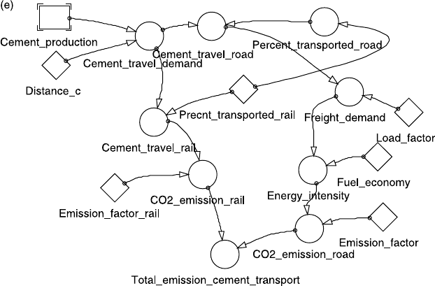
4. Model validation

Conﬁdence in the SD model for the system under study is

established through its validation on the basis of the data

utilized. The validation is carried out under three categories,

viz. historical validation of the data, a structural veriﬁcation

test and a dimensional consistency test.

For the historical validation the cement production

variable is selected. Data for the year 1990 is incorporated

in the model and projections are made up to the year 2003.

The model results give good agreement with the actual

values, as is shown in Fig. 3. Points representing the actual

and model values of cement production show an overall

increasing trend. However, in the year 2000–2001, actual

annual production was negative. The fall in growth rate is

attributed to a recession in the demand (IIC, 2002), which

subsequently attained a positive growth.

The structural validation tests are applied at every stage of

the model building process to detect any structural ﬂaws in the

model. These tests were, therefore, made simultaneously

throughout the model building process. Initially, the model

projected total population keeping the present rates of

population growth and then switched over to the zero

population growth rates by the years 2020 and 2011 for the

population stabilisation scenarios S1 and S2 respectively. This

is veriﬁed in Fig. 4 from the results obtained by running the

model.

Fig. 4. Projections for population of India under the baseline scenario (BS),

scenario 1 (S1) and scenario 2 (S2).

Fig. 3. Comparison of the quantity of cement production with the model

projections.

S. Anand et al. / Journal of Environmental Management 79 (2006) 383–398 391

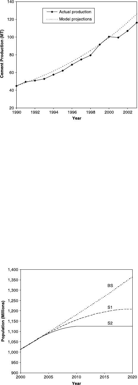
5. Sensitivity analysis

Sensitivity tests basically ascertain whether or not minor shifts

in the model parameters can cause shift in the behaviour of the

model. Once the robustness of the model is ensured, the model

can be used for policy making (Forrester, 1961; Mohapatra et al.,

1994). As already discussed, the emissions of CO

from the

cement industry are dependent on population, GDP, cement

demand and production. The sensitivity of the model to these

parameters is described in the following sections:

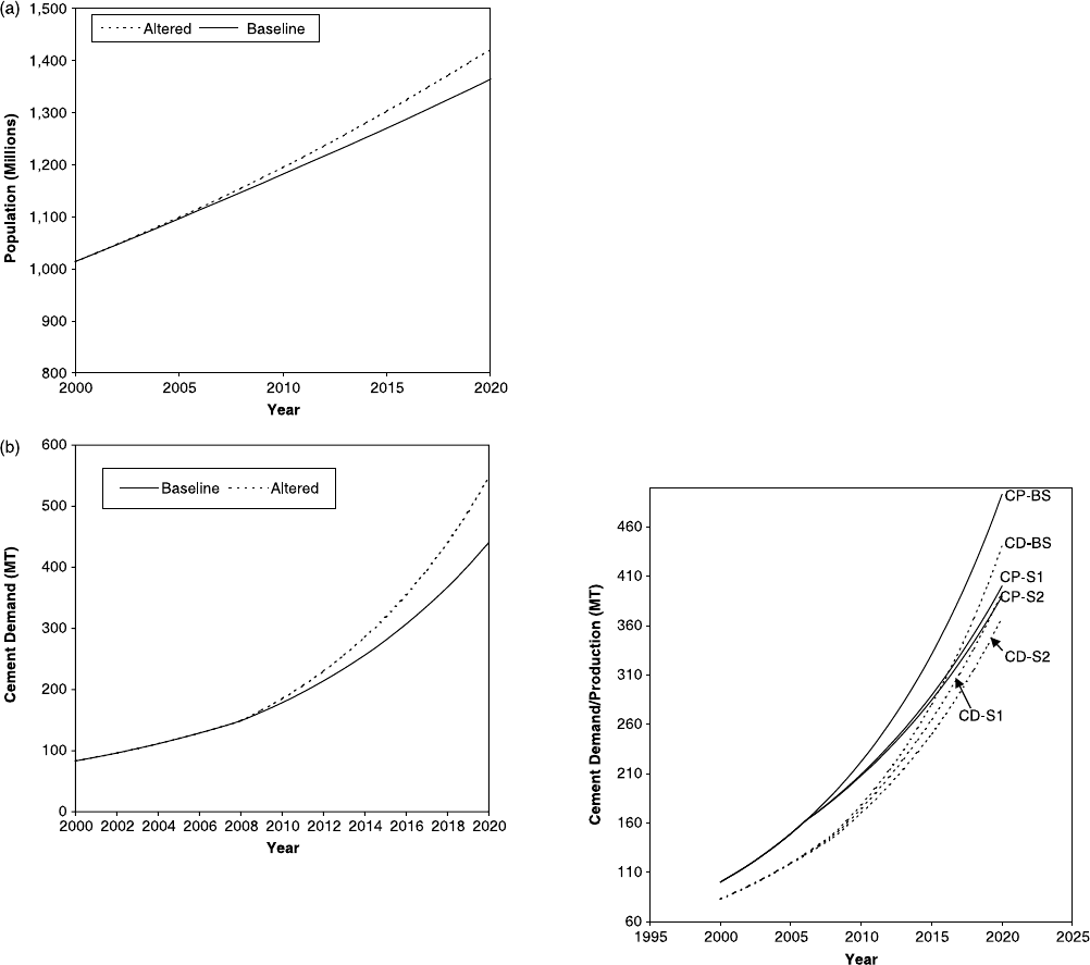
5.1. Impact of population on cement demand

Population is considered to play an important role in

controlling the cement demand, which in turn is the prime

determinant for the production of cement and the ultimate CO

emissions from the cement plants. It is evident from Fig. 5 (a)

that the population of the country would rise to 1421.80 million

from the projected ﬁgure of 1364.50 million, by the year 2020.

These calculations are made by changing the population

growth rate multipliers from 1.57, 1.50 and 1.44 to 1.63%, 1.7

and 1.76% for the years 2001–2006, 2006–2011 and 2011–

2018, respectively.

5.2. Impact of GDP on cement demand

The impact of GDP enhancement on cement demand is tested

by raising the GDP to 0.1 from 0.08 for the years 2008 onwards.

Fig. 5(b) shows the baseline and the altered curves. A small

increase in GDP does contribute to the increased cement demand.

The model is thus sensitive to minor shifts in the parameters

ensuring its clearance of the sensitivity test.

6. Results and discussion

The results obtained for different scenarios developed in the

SD model are discussed to ascertain the impacts of various

policy options on CO

emissions from the cement industry in

India. Trends are evaluated for a 20 year span starting from the

year 2000.

6.1. Baseline scenario

The rates of population growth and GDP as applicable in the

year 2000 (GOI, 1997, 2001–2002) were kept constant for

working out the baseline scenarios. The tec hnology employed

in making cement was also kept unaltered. Using these options,

India’s population is projected to reach 1364.50 million by the

year 2020. Fig. 4 shows the population growth for the baseline

(BS) and scenarios S1 and S2. The cement demand and cement

production are shown in Fig. 6. Cement demand projected for

Fig. 6. Projections for cement demand (CD) and cement production (CP) for the

baseline scenario (BS), scenario 1 (S1) and scenario 2 (S2).

Fig. 5. Sensitivity of the model to the different parameters. (a) Impact of

population growth rate multiplier on population. The population growth rate

multiplier is changed from 1.57, 1.50 and 1.44% to 1.63, 1.7 and 1.76% for the

years 2001–2006, 2006–2011 and 2011–2018, respectively, for obtaining the

altered scenarios and (b) variation in cement demand with gross domestic

product (GDP). The GDP is raised to 0.1 from 0.08 for the years 2008 onwards

for obtaining the altered scenarios.

S. Anand et al. / Journal of Environmental Management 79 (2006) 383–398392

the year 2011 by our model is 195.50 million tones, and this is

comparable to that of Schumacher and Sathaye (1999) (200.5

million tones). The cement production is projected to reach

492.83 million tonnes by the year 2020 with 331.13 million

tonnes of OPC, 108.18 million tonnes of PPC and 53.52 million

tones of PSC. The clinker requirement will be 400.95 million

tonnes with respective shares of 314.58 million tonnes for

OPC, 70.31 million tonnes for PPC and 16.06 million tonnes

for PSC.

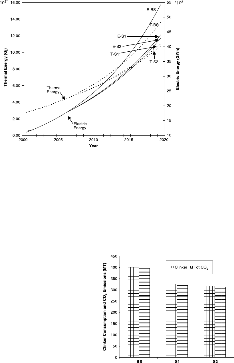
For the baseline scenarios the model has predicted that in

the year 2020, 13.5 9!10

Gj of thermal energy and

54211.49 GWh of electric energy will be required in the

making of cement. The respective CO

emissions will then be

135.92, 44.45 and 216.51 million tonnes from thermal energy

consumption, electric energy consumption and clinker con-

sumption. Figs. 7 and 8 show the annual growth of energy

utilization, clinker consumption and total CO

emissions,

respectively, for the BS and modiﬁed scenarios S1 and S2.

The direct CO

emissions are estimated to increase from

80.85 million tonnes in the year 2000–396.88 million tonnes in

20 years.

6.2. Modiﬁed scenarios

The cement demand and production are obviously linked to

the population growth, economic activity in the country, the

level and growth of GDP and the level of urbanization. Control

of the population growth can be one of the options for

mitigating the CO

emissions. As mentioned earlier, we have

analysed two scenarios. In scenario 1 the growth rate for

population is brought to zero by the year 2020 (S1) and in the

scenario 2 (S2) a faster decline in the growth rate is analysed

where zero growth rate is achieved in the year 2011.

Fig. 4 shows that with the S1 scenario the population of

India would reach 1208.38 million in the year 2020. The

cement demand will then be 393.31 million tonnes, a reduction

of 10.67% from the base line scenario. This is shown in Fig. 6.

Since the cement production is linked to its demand, which in

turn is linked to popul ation growth, a reduction of 18.81% in

production is projected as compared to the baseline scenario.

To produce the require d quantity of cement (400.12 million

Fig. 7. Projections for thermal (T-BS, T-S1/S2) and electric (E-BS, E-S1/S2) energy consumption for the baseline scenario (BS), scenario 1 (S1) and scenario 2 (S2).

Fig. 8. Projections for clinker consumption for cement production and total

emissions from the cement industry under the baseline scenario (BS),

scenario 1 (S1) and scenario 2 (S2) for the year 2020.

S. Anand et al. / Journal of Environmental Management 79 (2006) 383–398 393

tonnes), the consumption of thermal energy will be 11.04!

Gj, electricity 44012.70 GWh (Fig. 7) and the clinker

requirement will be 325.52 million tonnes (Fig. 8). As shown in

Fig. 8, 322.22 million tonnes of CO2 will be emitted in the year

2020 from a combination of thermal energy consumption

(110.35 million tonnes) electricity consumption (36.09 million

tonnes) and clinker consumption (175.78 million tonnes). A

further decrease in all the parameters, shown in Fig. 6–8,

obviously occurred when we tried to stabalise the rate of

population growth to zero by the year 2011 (S2). With the

scenario S2 the popul ation would stabalise at 1125.30 million

by the year 2011 and, therefore, remain constant. A reduction

of 20.92% (389.74 million tonnes) in cement produc tion is

projected for the year 2020 when applying the S2 policy option.

Accordingly, the consumption of thermal energy will be

10.75!10

Gj, ele ctricity use will be 423871.48 GWh and

317.08 million tonnes of clinker will be required. The

corresponding CO

emissions will be 107.49 million tonnes

due to thermal energy consumption, 35.15 million tonnes from

electricity consumption, and 171.22 million tonnes in the

calcination process. In total a 20.92% (313.87 million tonnes)

reduction in direct CO

emissions will occur. When we reduce

the rate of population growth, a decrease obviously occurs in

the cement demand and produc tion. But, the decline in cement

demand does not follow the trend of population decrease, as the

cement demand is linked to the investment in the cement-

intensive infrastructure. India being a developing country such

an investment will increase.

6.2.1. Energy management scenario

Fig. 9 shows the outcome of the energy management policy

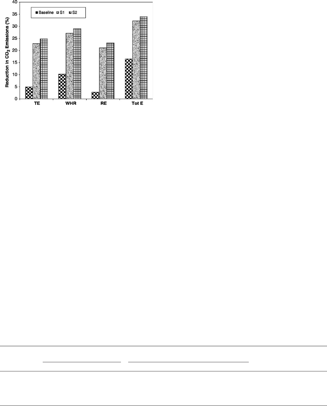
options for the BS and S1 and S2 scenarios. If 30% thermal

energy from the waste heat is taken into account, the CO

emissions would decline to 356.11, 289.12 and 281.62 million

tonnes for the BS, S1 and S2, respectively. The CO

emissions

would be substantially curtailed by meeting some of the

electric energy demand in the cement plants with renewable

energy. It is expec ted that the renewable energy resources will

play an important role in the years to come. For analyzing the

effect of renewable energy we have replaced 25% of the

electric energy supply to the cement plants with renewable

energy. This is incorporated from the year 2010 sinc e the

electric power generation from renewable energy resources is

expected to play a substantial role by that time. Reductions of

2.80% for BS, 21.09% for S1 and 23.13% for S2 in CO

are

projected under these conditions. It is worth mentioning here

that four cement plants in the Southern part of India have

already installed 80.25 MW (e) capacity wind power gen-

erators in their wind farms. Presently they feed their output into

the grid (www.cleantechindia.com/eicnew/cement.html).

Energy efﬁcient clin ker making tech nology is now

available. When the improved speciﬁc energy consumption

of 2.9 Gj/tonne of clinker production in the plant for the best

practice technology (Schumacher and Sathaye, 1999; Price

et al., 2000) is considered, CO

emissions are reduced by 4.95,

22.83 and 24.83% for the BS, S1 and S2. Fig. 9 also shows the

percent reduc tions in theCO

emissions for an integrated

scenario where all the above-mentioned energy management

options are implemented simultaneously.

Fig. 9. Per cent reductions in CO

emissions from cement industry for the

energy efﬁciency improvement (EEI) scenarios; 25% contribution of electric

energy from the renewable sources of energy (RE) starting from the year 2010,

30% thermal energy recovery from waste heat (WHR), 2.9 Gj/tonne speciﬁc

energy consumption (T) is used in clinker processing and a combined scenario

taking all the above mentioned energy efﬁciency improvement scenarios (TotE).

The baseline scenario (BS), scenario 1 (S1) and scenario 2 (S2) are shown

separately.

Table 1

Projections of CO

emissions due to clinker consumption for increasing share of Ordinary Portland Cement (OPC), Portland Slag Cement (PSC) and Portland

Pozzolana Cement (PPC) for the baseline scenario

Year Availability of blending materials

(million tonnes)

Share of cement types (million tonnes) CO

emissions from clinker

consumption (million tonnes)

Fly ash Slag OPC PSC PPC

2000 28.15 15.91 67.46 10.90 22.04 44.11

2005 36.76 21.41 100.41 16.23 32.80 65.65

2010 48.00 28.81 149.46 24.16 48.83 97.72

2015 62.67 38.78 222.47 35.96 72.68 145.46

2020 81.83 52.19 331.13 53.52 108.18 216.51

WHR, Waste heat recovery; in this scenario 30% of the thermal energy is recovered from the waste heat. SM, Structural management; in this case the share of

blended cement is increased to 37% OPC, 45% PPC, 16% PSC and 2% ZP.BS, Baseline scenario. S1, Population growth is stabilised to zero by the year 2020. S2,

Population growth is stabilised to zero by the year 2011.The share of blended cements is ascertained from the availability of ﬂy ash and slag.

S. Anand et al. / Journal of Environmental Management 79 (2006) 383–398394

6.2.2. Structural management scenario

For the structural management scenario the share of PPC

has been increased to 45%, PSC to 16% and zeolite Portland to

2%. Availability of ﬂy ash and blast furnace slag would restrict

the further increase of their share.

In India the coal consumption in thermal power plants was

234.6 million tonnes in the year 2000 and is projected to reach

681.92 million tonnes by the year 2020. Therefore, 28.15

million tonnes of ﬂy ash was available for cement use in the

year 2000, but actually merely 6.61 million tonnes was utilized.

The ﬂy ash demand in cement plants is projected to reach 66.53

million tonnes in the year 2020 and 81.83 million tonnes will

be available. Table 1 gives the projections of the availability of

blending materials and CO

emissions for structurally modiﬁed

cement production. Pig iron production in the iron and steel

industry was 20.5 million tonnes in the year 2000, thereby

generating 15.91 million tonnes of blast furnace slag. This iron

production would reach 67.25 million tonnes in the year 2020

generating 52.19 million tonnes of furnace slag. With the

presently chosen policy options the cement industry would

require 51.25 million tonnes of slag. This goes well with its

availability.

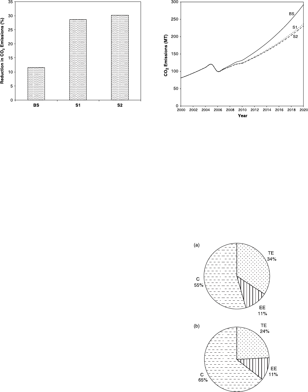
Scenarios generated by enhancing the percentages in

blended cement to 45% PPC, 16% PSC and 2% zeolite

Portland lead to 333.69 million tonnes of clinker consumption

and 11.81!10

Gj thermal energy consumption by the year

2020. This option amounts to 11.63% reduction in the CO

emissions for the baseline scenario. Along the same lines, a

further reduction of 28.26 and 30.12% is expected for S1 and

S2, respectively, as is shown in Fig. 10. A decline in the share

of OPC production from 62% to 56% and increase in the share

of PPC production from 26 to 32% has been reported for the

year 2001–2002 (http://www.indiacements.co.in/industry-

Ver2.asp). Thus the usage of blended cements can be

increased.

Structural change is beneﬁcial not only in reducing the

limestone consumption and its inherent carbon release but also

in reducing the energy related CO

emissions.

6.2.3. Integrated scenario

A combined scenario is generated by integrating the strategy

of structural management (2% zeolite Portland, 45% PPC, 16%

PSC and 37% OPC) and energy management (30% therm al

energy recovered from waste heat, 25% of electric energy from

renewable energy resources and taking 2.9 Gj/tonne speciﬁc

energy consumption). For this integrated scenario, shown in

Fig. 11, in the year 2020 the CO

emissions are projected to

decrease by 26.37% (292.23 million tonnes), 40.22% (237.25

million tonnes) and 41.77% (231.11 million tonnes) for the BS,

Fig. 10. Per cent reductions in CO

emissions for the structural management

scenario under the baseline scenario (BS), scenario 1 (S1) and scenario 2 (S2).

Fig. 11. Annual projections of the cumulative effect of the energy efﬁciency

improvement scenario and structural management scenario on CO

emissions

under the baseline scenario (BS), scenario 1 (S1) and scenario 2 (S2).

Fig. 12. Per cent share of CO

emissions from the use of clinker (C), electric

energy (EE) and thermal energy (TE) for (a) the baseline scenario and (b)

integrated scenario S2.

S. Anand et al. / Journal of Environmental Management 79 (2006) 383–398 395

S1 and S2, respectively. There is a kink in Fig. 11

corresponding to the year 2006. This is due the incorporation

of policy options implemented from the year 2006 (except for

the 25% share from renewable energy). The renewable energy

is made effective from the year 2010, which is evident in the

form of another small kink.

Reductions in the CO

emissions are attributed to the

combined effect of all the mitigation options. The shares of

emissions from the use of clinker, electric energy and

thermal energy for the BS and S2 scenarios are shown in Fig. 12.

In the case of BS, out of the total 396.88 million tonnes CO

emissions, 216.51 million tonnes comes from the clinker

consumption. This is 55% of the total share. In the case of

integrated scenario S2 the share of the CO

emissions (231.11

million tonnes) from clinker increases to 65%. However, the

percent share of CO

emissions from the thermal energy reduces

to 24% (55.46 million tonnes) for the integrated scenario S2.

6.2.4. Indirect CO

emissions

The indirect contribution to the CO

emissions from

cement industry related operations comes from the fossil-

fuel combustion in transporting the raw materials (coal and

limestone) to the industry and the ﬁnished product cement

to the market. For the year 2000, a total of 2.24 million

tonnes of CO

is estimated to have been released in

transporting coal to the cement industry. In this the share

from road transportation is 2.01, and 0.40 million tonnes are

from rail transport. This value is projected to reach 11.87,

9.64 and 9.39 million tonnes for the BS and S 1 and S2,

respectively, by the year 2020.

The impact of policy options on the percent reduction of

indirect CO

emissions from transport of the raw material

(limestone and coal) to the cement plants is shown in Table 2.

When the share of blended cement is increased, the coal

transport related CO

emissions come down. On increasing the

share of blended cement to 37% OPC, 45% PPC, 16% PSC and

2% zeolite Portland, emission reductions of 13.06, 29.46 and

31.26% for the BS, S1 and S2, respectively, are expected by the

year 2020. This is due to the reduced fuel requirement in the

case of blended cement. If the energy efﬁciency of the plants

could be improved to 2.9 Gj/tonne of clinker, a maximum

reduction of 32.35% in the CO

emissions for S2 is expected,

due to lowering of the coal consumption. In a combined

scenario of structural management and energy efﬁciency

improvement, the CO

emissions from the coal transport

come down by 58.80%. The CO

emissions from the transport

of limestone to the cement plants are projected to reach 12.66,

10.28 and 10.01 million tonnes by the year 2020 for the BS, S1

and S2, respectively.

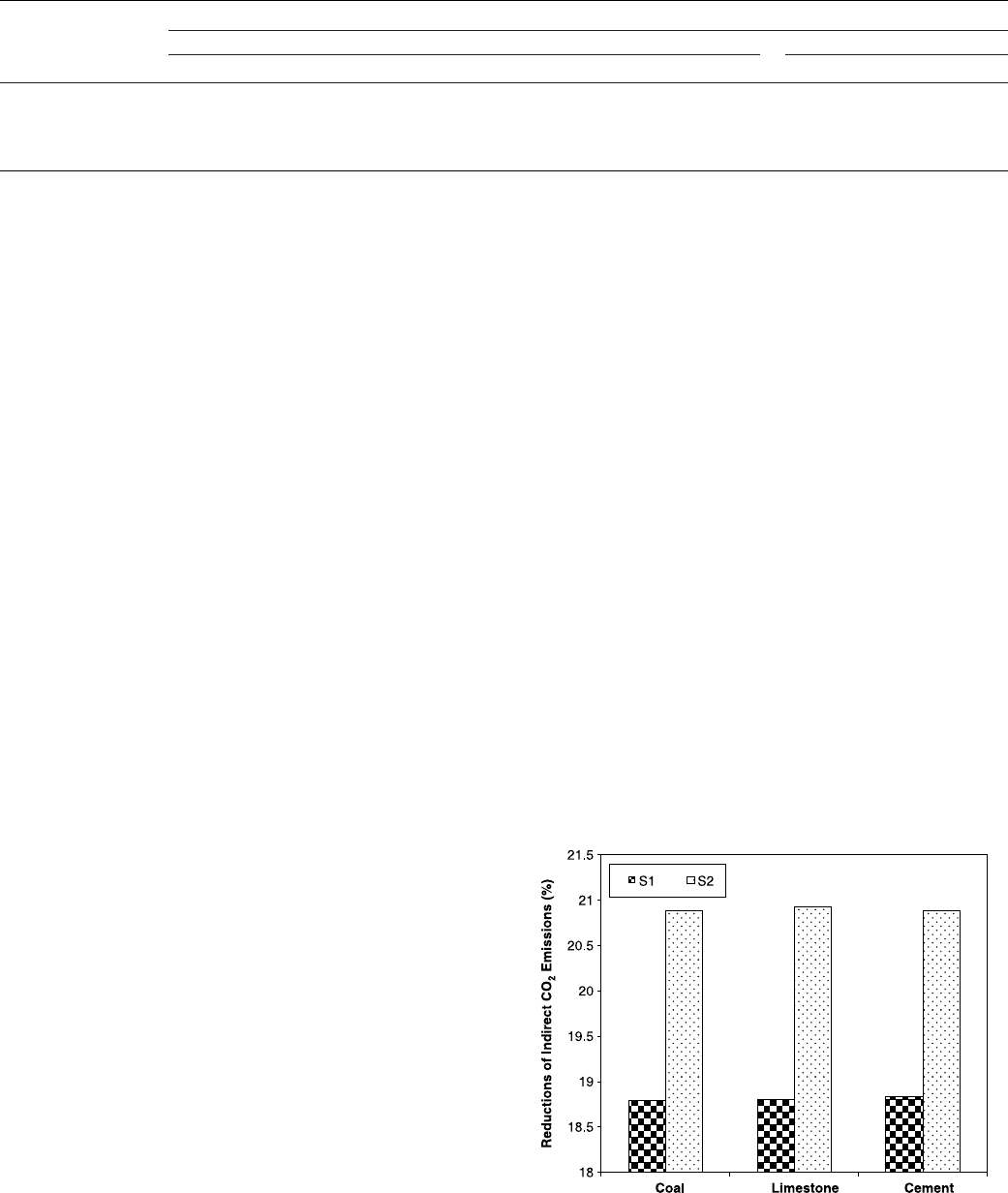
In the baseline scenario transport of cement to the market

will contri bute 12.16 million tonnes of CO

emissions by the

year 2020. These emissions are estimated to go down to the

respective values of 9.87 and 9.62 million tonnes for

population growth stabalisation scenarios S1 and S2. Percent

reductions of indirect vehicular CO

emissions from the

transport of the raw materials (coal, limestone) to the cement

plants and cement to the market are shown in Fig. 13.

Emissions from the transportation of the materials by

road are obviously more than those by rail transport.

Railways consume the least direct fuel energy per tonne

kilometer and hence less CO

is emitted per tonne

kilometer. A reduction of approximately 85% in the CO

emissions is estimated if the freight transportation is shifted

from road to rail. Ramanathan and Parikh (1999) have

reported that the energy consumption and CO

emissions

per tonne kilometer by trucks are nearly ﬁve times the

corresponding values for rail transport.

Table 2

Impact of policy options on the reduction of indirect CO

emissions from raw material (limestone and coal) transport to the cement plants

Policy options Reduction of indirect (vehicular) CO

emissions from raw material transport (%)

Coal Limestone

BS S1 S2 BS S1 S2

TEEI 14.41 30.50 32.35 0.0 18.80 20.93

WHR 30.00 43.13 44.65 0.0 18.80 20.93

SM 13.06 29.40 31.26 13.11 29.46 31.28

TEEICWHRCSM 47.94 57.70 58.80 13.11 29.46 31.28

TEEI, Thermal energy efﬁciency improvement scenario where the speciﬁc energy consumption is decreased to 2.9 Gj/tonne cement production.

Fig. 13. Per cent reductions in indirect (vehicular) CO

emissions from transport

of the raw material (limestone and coal) to the cement plants and ﬁnished product

cement to market under the Scenario 1 (S1) and scenario 2 (S2).

S. Anand et al. / Journal of Environmental Management 79 (2006) 383–398396

7. Conclusi ons

A system dynamics model for the CO

emissions from the

cement sector was developed. The model was applied to make

projections of CO

emissions in India for a time span of 20

years. The cement production with the baseline scenario

(present rate of population growth) is projected to contribute

396.89 million tonnes of CO

to the greenhouse gas load by the

year 2020. Mitigation strategies for curtailing the CO

emissions from this sector are identiﬁed and analysed. The

emissions from cement plants are dependent on many

interrelated variables, viz. population and GDP growth rate,

cement demand and production, clinker consumption and

energy utilized. Quantitative estimates of CO

emissions due to

stabilisation of the population growth, curtailment of excess

cement production, structural management, energy efﬁciency

management and a combination of all these measures have

been worked out. A combined scenario with population

stabilisation by the year 2010, structural shifting (2% zeolite

Portland, 4 5% PPC, 16% PSC and 37% OPC), 25%

contribution from renewable sources of energy for the cement

industry starting from the year 2010, and use of an energy

efﬁcient process with 2.9 Gj/tonne speciﬁc energy consumption

and 30% thermal energy recovery from waste heat can reduc e

the CO

emissions from the Indian cement industry by

approximately 42% in the year 2020. This could be a

substantial lowering of the greenhouse gas load to the

environment.

Indirect CO

emissions coming from the transportation of

raw materials (coal and limestone) to the cement plants and

ﬁnished products (cement) to the market were also worked out.

The CO

emissions from road transport are more in comparison

to that from rail transport. Th us, a shift from the use of trucks to

the railways will also lead to a reduction in CO

emissions.

Acknowledgements

One of the authors (S.A.) thanks the Indian Institute of

Technology Delhi for the award of fellowship to carry out this

research work.

References

Anand, S., Dahiya, R.P. and Vrat, P. (2005) Investigations of methane

emissions from rice cultivation in Indian context. Environment Inter-

national 31, 469-482 (www.elsevier.com/locate/envint).

CEMBUREAU, 1996. Word Cement Directory, CEMBUREAU. The European

Cement Association, Brussels, Belgium.

CEMBUREAU, 1998. Cement Production, Trade, Consumption, Data: World

Cement Market in Figures 1913–1995, World Statistical Review 18.

CEMBUREAU—The European Cement Association, Brussels, Belgium.

CEMBUREAU, 1999. Cement Production, Trade, Consumption Data: World

Cement Market in Figures 1913–1995, World Statistical Reviews 19 and

20. CEMBUREAU—The European Cement Association, Brussels,

Belgium.

Choudhary, R., Bhakatvatsalam, A.K., 1997. Beneﬁcation of Indian coal by

chemical techniques. Energy Conversion and Management 38 (2), 173–

178.

CII, 1995. Speciﬁc energy consumption norms in India: Cement industry,

Chennai. Confederation of Indian industry.

Ford, A., 1996. Testing snake river explorer. System Dynamics Review 12,

305–329.

GHG Protocol-Mobile Guide, 2001. Calculating CO2 emissions from mobile

sources. Guidance to calculation worksheets (www.ghgprotocol.org/

standard/mobile.doc).

Government of India, 1997. Report to the Planning Commission. 9th Five

Year Plan, 1. (http://www.developmentﬁrst.org/India/planning-commis-

sion/9thfyp/FYPVol1.pdf).

Government of India, 2001–2002. Economic Survey. Ministry of Finance.

(http://indiabudget.nic.in/es2001-02/).

Guneralp, B., Barlas, Y., 2003. Dynamic modelling of a shallow fresh water

lake for ecological and economic sustainability. Ecological Modelling 167,

115–138.

Guo, H.C., Liu, L., Huang, G.H., Fuller, G.A., Zou, R., Yin, Y.Y., 2001. A

system dynamics approach for regional environmental planning and

management. A study for the lake Erhai Basin. Journal of Environmental

Management. 61, 93–111, www.idealibrary.com.

Hendriks, C.A., Worrell, E., Price, L., Martin, N., Ozawa Meida, L.,

1999. Greenhuse gases from cement production. IEA Greenhouse Gas

R & D Programme. Report # PH 3/7. Ecofys, Utrecht, The

Netherlands.

IIC, 2002. Industry, Finance and Business. International Investment Centre

Monthly Newsletter (July) (http://iic.nic.in/ifb0702.htm).

International Energy Agency, 1999. The reduction of greenhouse gas emissions

from the cement industry, Report PH 3/7, Paris, France.

Karavezysis, V., Timpe, K.P., Marzi, R., 2002. Application of system dynamics

and fuzzy logic to forcasting of municipal solid waste. Mathematics and

Computers in Simulation 2071, 1–10.

Karwa, D.V., Sathaye, J., Gadgil, A., Mukhopadhyay, M., 1998. Energy

efﬁciency and environmental management options in the cement Industry.

ADB Technical Assistance Project (TA:2403-IND). ERI, Forest Knolls,

Calif.

Khurana, S., Khurana, S., Banerjee, R., Gaitonede, U., 2002. Energy balance

and cogeneration for a cement plant. Applied Thermal Engineering 22,

485–494.

Marchal, G., 2001. Decreasing pollution. Cement and Building Materials

Review (3) (AUCBM).

Mashayekhi, A.N., 1993. Transition in New York state solid waste system: a

dynamic analysis. System Dynamics Review 9, 23–48.

McCaffrey, R., 2001. Climate change and the cement industry. GCL: Global

Cement and Lime Magazine (www.probubs.com/climate/climate.html.).

Mehra, M., Damodaran, M., 1993. Anthropogenic emissions of greenhouse

gases in India (1989–90), The Climate Change Agenda: An Indian

Perspective. Tata Energy Research Institute, New Delhi, India.

Mohapatra, P.K.J., Mandal, P., Bora, M.C., 1994. Introduction of System

Dynamics Modelling. Orient Longman Hyderabad, India.

Naill, R.F., Gelanger, S., Klinger, A., Petersen, E., 1992. An analysis of cost

effectiveness of US energy policies to mitigate global warming. System

Dynamics Review 8, 111–118.

Price, L., Worell, E., Martin, N., Lehman, B., Sinton, J., 2000. China’s

industrial Sector in an International Context. Proceedings of the Workshop

on ‘Learning from International Best Practice Energy Policies in the

Industrial Sector’, Bejing, China, 22–23. http://eetd.lbl.gov/ea/ies/suni6/

industry46273.pdf.

Ramanathan, R., Parikh, J.K., 1999. Transport sector in India: an analysis in the

context of sustainable development. Transport Policy 6, 35–45.

Saysel, A.K., Barlas, Y., Yenig, O., 2002. Environmental sustainability in an

agricultural development project: a system dynamics approach. Journal of

Environmental Management, 64, 247–260http://www.idealibrary.com.

Schumacher, K., Sathaye, J., 1999. India’s cement industry: Productivity,

energy efﬁciency and carbon emissions. LBNL-41842. Lawrence Berkley

National Laboratory, USA. http://eetd.lbl.gov/ea/ies/suni6/industry41842.

pdf.

Somani, R.A., Kothari, S.S., 1997. Die Neue Zementlinie bei Rajashree

Cement in Malkhed/Indien. ZKG International 8, 430–436.

S. Anand et al. / Journal of Environmental Management 79 (2006) 383–398 397

TEDDY 2000/2001. TERI Energy Data Directory & Yearbook, Pub: Tata

Energy Research Institute, New Delhi.

Vizayakumar, K., Mohapatra, P.K.J., 1991. Environmental impact analysis of a

coalﬁeld. Journal of Environment Management 34, 73–93.

Vizayakumar, K., Mohapatra, P.K.J., 1993. Modelling and simulation of

environmental impacts of coalﬁeld: system dynamics approach. Journal of

Environmental Systems 22, 59–73.

Vrat, P., Gupta Y.K., Gupta, A., 1993. A System dynamics study of

global warming. Proceedings of xviith National System Conference,

Kanpur.

World Energy Council, 1995. Energy efﬁciency improvement utilising high

technology: an assessment of energy use in industry and buildings. Prepared by

Marc D. Levine, Lynn Price, Nathan Martin and Ernst Worrell, WEC, London.

Worrell, E., Smit, R., Phylipsen, D., Blok, K., Vleuten, F., Jansen, J., 1995.

International comparison of energy efﬁciency improvement in the cement

industry. In: Summer Study on Energy Efﬁciency in Industry, ACEEE

proceedings, Washington, DC.

Wu, J., Barlas, Y., Wankat, J.L., 1993. Effect of patch connectivity and

arrangement on animal metapopulation dynamics: a simulation study.

Ecological Modeling 65, 221–254.

S. Anand et al. / Journal of Environmental Management 79 (2006) 383–398398